
반응형
SVM을 통한 구매 가능성이 있는 고객 분류하기
이 포스팅은 앞선 K-NN을 통한 구매 가능성이 있는 고객 분류하기와 같은 자료를 사용하지만 다른 머신러닝을 통해 분류를 해 볼 것이다.
import numpy as np
import matplotlib.pyplot as plt
import pandas as pd
from sklearn.preprocessing import StandardScaler
from sklearn.model_selection import train_test_split
from sklearn.svm import SVC
from sklearn.metrics import confusion_matrix
라이브러리 import
df = pd.read_csv('Social_Network_Ads.csv')
df.head()
df.info()
df.isna().sum()
df.describe()
csv데이터를 가져오고, 자료를 확인한다.


X = df.iloc[:, [2,3]]
y = df['Purchased']

X.head()
y
X와 y를 설정해준다.


sc = StandardScaler()
X = sc.fit_transform(X)
X
X를 피쳐스케일링한다

X_train, X_test, y_train,y_test = train_test_split(X,y,test_size = 0.2, random_state = 0 )
X.shape			#(400, 2)
X_train.shape	#(320, 2)
X_test.shape	#(80, 2)
테스트 셋과 트레이닝 셋으로 나누어주고, shape을 확인한다.
classifier = SVC(kernel='linear', random_state=0)
classifier.fit(X_train, y_train)
y_pred = classifier.predict(X_test)
y_pred
X의 테스트 셋을 통해 y를 예측했다.
y_test = y_test.values
이제 y_pred와 y_test를 비교하여 성능을 측정한다.
cm = confusion_matrix(y_test, y_pred)
cm
정확도 = (cm[0][0]+cm[1][1])/cm.sum()
여기서부터는 유용한 코드
from matplotlib.colors import ListedColormap
X_set, y_set = X_test, y_test
X1, X2 = np.meshgrid(np.arange(start = X_set[:, 0].min() - 1, stop = X_set[:, 0].max() + 1, step = 0.01),
                     np.arange(start = X_set[:, 1].min() - 1, stop = X_set[:, 1].max() + 1, step = 0.01))
plt.contourf(X1, X2, classifier.predict(np.array([X1.ravel(), X2.ravel()]).T).reshape(X1.shape),
             alpha = 0.75, cmap = ListedColormap(('red', 'green')))
plt.xlim(X1.min(), X1.max())
plt.ylim(X2.min(), X2.max())
for i, j in enumerate(np.unique(y_set)):
    plt.scatter(X_set[y_set == j, 0], X_set[y_set == j, 1],
                c = ListedColormap(('red', 'green'))(i), label = j)
plt.title('K-NN (Test set)')
plt.xlabel('Age')
plt.ylabel('Estimated Salary')
plt.legend()
plt.show()
from matplotlib.colors import ListedColormap
X_set, y_set = X_train, y_train
X1, X2 = np.meshgrid(np.arange(start = X_set[:, 0].min() - 1, stop = X_set[:, 0].max() + 1, step = 0.01),
                     np.arange(start = X_set[:, 1].min() - 1, stop = X_set[:, 1].max() + 1, step = 0.01))
plt.contourf(X1, X2, classifier.predict(np.array([X1.ravel(), X2.ravel()]).T).reshape(X1.shape),
             alpha = 0.75, cmap = ListedColormap(('red', 'green')))
plt.xlim(X1.min(), X1.max())
plt.ylim(X2.min(), X2.max())
for i, j in enumerate(np.unique(y_set)):
    plt.scatter(X_set[y_set == j, 0], X_set[y_set == j, 1],
                c = ListedColormap(('red', 'green'))(i), label = j)
plt.title('K-NN (Training set)')
plt.xlabel('Age')
plt.ylabel('Estimated Salary')
plt.legend()
plt.show()
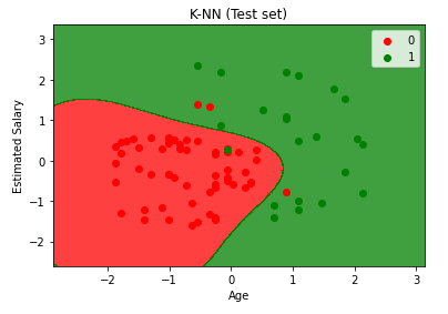
from matplotlib.colors import ListedColormap
X_set, y_set = X_test, y_test
X1, X2 = np.meshgrid(np.arange(start = X_set[:, 0].min() - 1, stop = X_set[:, 0].max() + 1, step = 0.01),
                     np.arange(start = X_set[:, 1].min() - 1, stop = X_set[:, 1].max() + 1, step = 0.01))
plt.contourf(X1, X2, classifier2.predict(np.array([X1.ravel(), X2.ravel()]).T).reshape(X1.shape),
             alpha = 0.75, cmap = ListedColormap(('red', 'green')))
plt.xlim(X1.min(), X1.max())
plt.ylim(X2.min(), X2.max())
for i, j in enumerate(np.unique(y_set)):
    plt.scatter(X_set[y_set == j, 0], X_set[y_set == j, 1],
                c = ListedColormap(('red', 'green'))(i), label = j)
plt.title('K-NN (Test set)')
plt.xlabel('Age')
plt.ylabel('Estimated Salary')
plt.legend()
plt.show()
from matplotlib.colors import ListedColormap
X_set, y_set = X_train, y_train
X1, X2 = np.meshgrid(np.arange(start = X_set[:, 0].min() - 1, stop = X_set[:, 0].max() + 1, step = 0.01),
                     np.arange(start = X_set[:, 1].min() - 1, stop = X_set[:, 1].max() + 1, step = 0.01))
plt.contourf(X1, X2, classifier2.predict(np.array([X1.ravel(), X2.ravel()]).T).reshape(X1.shape),
             alpha = 0.75, cmap = ListedColormap(('red', 'green')))
plt.xlim(X1.min(), X1.max())
plt.ylim(X2.min(), X2.max())
for i, j in enumerate(np.unique(y_set)):
    plt.scatter(X_set[y_set == j, 0], X_set[y_set == j, 1],
                c = ListedColormap(('red', 'green'))(i), label = j)
plt.title('K-NN (Training set)')
plt.xlabel('Age')
plt.ylabel('Estimated Salary')
plt.legend()
plt.show()
반응형
'미니프로젝트' 카테고리의 다른 글
| CNN을 활용하여 드론과 새 분류하기 (4) | 2021.04.04 |
|---|---|
| 구글에서 파이썬 셀레니움을 통한 이미지 크롤링 (0) | 2021.04.02 |
| 공항 기상 시각화 (0) | 2021.04.01 |
| 인천 1호선 일자 및 시간대별 승하차 현황 시각화/prophet을 통한 승객 수요 예측 (0) | 2021.04.01 |
| K-NN을 통해 구매 가능성이 있는 고객 분류하기 (0) | 2021.04.01 |